June 27, 2014 / by Christina Schneider / / @
Using logs to predict the future
We collect a lot of search data from our portals. Millions of entries show what people have searched for and when.
The interesting question for us is: Can we use this data to be able to give our customers better recommendations at the right time?
Motivation
To be able to react correctly to upcoming season changes and annual events is very important for us. When do our customers mainly search for sandals and when for curtains? Whats the best time to advertise evening gowns?
Let’s say we have collected data covering just over two years for the frequently searched term Sandalen. What are the steps compute a prediction model and predict the next months?
Prediction
For the prediction the open-source data analysis tool KNIME was used.
It provides a modular set of different algorithms and preprocessing steps which can be combined freely, so the workflow can be adjusted exactly to ones needs.
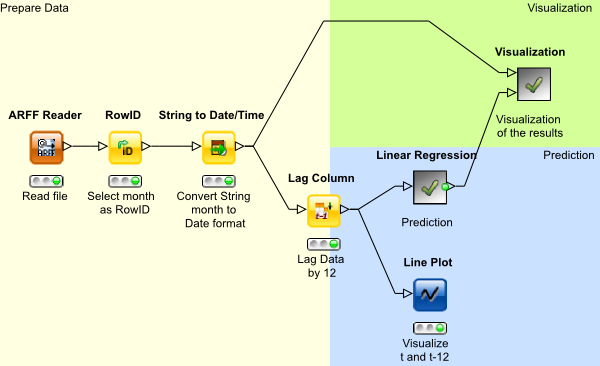
Here you can see the main steps taken.
Preprocessing
In the preparation step the data is fed into the workflow as an .arff file. Some basic steps are taken to prepare the data for prediction. The month is set as the RowID, which later will be our x-axis in the graph. Then the month is converted to a Date format which KNIME can handle.
Make it comparable
The first step is to normalize the data. This helps comparing the trend curves of different search terms to each other. Plotting this data you can easily see which terms follow the same annual pattern.
This was already done in the .arff file, but can easily be done by adding a normalize step to the KNIME workflow.
The past is the future
Now comes the interesting part - “Lag Column”.
To be able to handle seasonality regarding the prediction with linear Regression KNIME offers using lags.
Essentially you take the data from one year and subtract the values from the previous year, which gives us a lag of 12 in this example.
Whats left is just the change in comparison to the previous year, seasonality removed. Now you can predict the trend of the curve left and add the seasonality at the end.
A look ahead
For the prediction part the computed seasonality part needs to be removed first. For each data point the value of the data point 12 months ahead is subtracted.
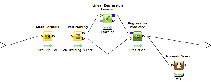
As we have 28 data points in total and want to see how the prediction performed in the end, we split the data into a training and a test set. We take 20 data points for training and predict the next 8 data points.
The linear Regression algorithm computes a model using the training data and calculated the prediction. The results can be compared to the test data.
Result
Let’s look at what we’ve got:
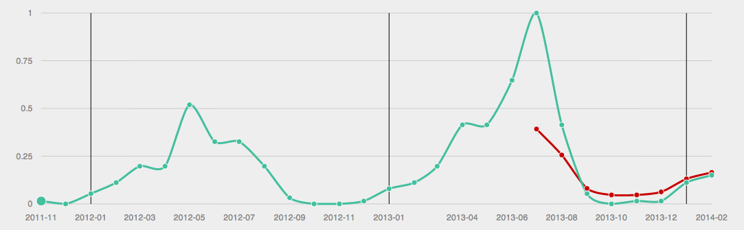
The green line represents the original data and the red one are our predicted data points.
Plotting the data you can clearly see the seasonality changes. The predicted data points are pretty close to the original data points. The main difference is between the original data point for July and the predicted one. This is due to the fact that in the year 2012 the peak of searches for sandals was more into May, whereas for 2013 it is moved to June and July.
Using more training data such differences in seasonality between the years can be compensated. With more data you can not only subtract the value of the previous year, but the average of the previous years, to remove the seasonality from the training data. This should give a much better prediction and be less vulnerable to variations of the seasonal pattern over the years.
Lessons learned
Lots of logged data can be a programmers heaven and hell at the same time. If you want to predict seasonal changes you need data which covers a period of more than a year, better several years.
At the same time data from several years is a lot to process.
So the challenge is to reduce the amount of data you need to process without loosing too much information.